| Page |
|
Plotting a Moving Average Graph
The moving-average values are plotted using similar axes to the original time-
series graph. Each moving-average value is plotted at the mid-point of the
period to which it refers. In the Electrical Use graph, the first moving average
(665 units) is from quarter 1 to quarter 4 in 2000. This was plotted midway
between quarters 1 and 4 (at 2.5). Check this out on the graph below. The
second average (657.5) is plotted midway between quarters 2 and 5, and so on.
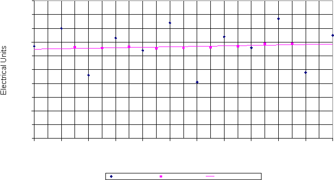
Comparison of the Raw Data and Moving Average Graphs
The plotted points from the original time-series graph and the moving-average
graph are both shown on the graph below. They are both time-series graphs –
the essential difference is that the original used the raw quarterly data whereas
the second used the averaged data. The trend, shown by the line of best fit, can
be compared directly with the original time-series plot.
The line of best fit shows a gradual increase in the use of electricity over the 3
years. Notice that the trend line has been extended back to the first quarter and
also continues beyond the last average point to the last quarter. By extending the
trend line you can make an estimate of values that lie outside the range of data.
In Exercise 2 you are expected to plot moving average points and draw the line
of best fit by hand.
Time-Series Raw Data and 4-Point Moving Averages
0
100
200
300
400
500
600
700
800
900
1000
1
2
3
4
5
6
7
8
9
10
11
12
Quarters
Time-Series Data
Moving Averages
"Best Fit" Trend Line